Dorado v2.0.0 part 3: methylation
•


This post follows my last two posts on Dorado v2. Read those to catch up!
In this third installment, I’m going to examine methylation calling.1 In their London Calling 2026 tech talk, ONT said hac@v6.0.0 has ‘improvements in all modified base accuracies’.2 Here is a quote from that presentation:
With hac v6, we deliver the most accurate modified basecalling ever produced, outperforming sup on every single model.
Using the same genomes from the previous posts, I’m going to see how the different basecalling models do with methylation calling in bacteria.
Models
When dorado basecaller uses a base modification model, this runs as an extra pass on each read after normal basecalling. The basecalled sequence and raw-signal context are given to another neural network which gives a modification probability for each candidate base. This is then stored in the read BAM file in the MM and ML tags.3
For my data, I looked for the mods most common in bacteria: 6mA, 5mC and 4mC. Each of the three tested basecalling models has a modified-base model for 6mA and another that does both 4mC and 5mC: hac@v5.2.0_6mA@v1, hac@v5.2.0_4mC_5mC@v1, hac@v6.0.0_6mA@v1, hac@v6.0.0_4mC_5mC@v1, sup@v5.2.0_6mA@v1 and sup@v5.2.0_4mC_5mC@v1. These all have ~3.2 million parameters and use the same architecture: CNN processing of signal and sequence context, a merge convolution and two 384-dimensional LSTM layers.
I did not test the 5mC_5hmC model, since 5hmC modification is not common in bacteria (though it can occur in phages). And I didn’t test the 5mCG_5hmCG model, since CpG methylation is more of an animal thing.
Methods
My goal here is to compare how the different basecalling models (hac@v5.2.0, hac@v6.0.0 and sup@v5.2.0) perform with modified basecalling. I ran each of the five genomes through this simple modkit analysis:
dorado aligner reference.fasta reads.bam | samtools sort > alignments.bam
samtools index alignments.bam
modkit pileup alignments.bam modkit.bed --modified-bases 6mA 5mC 4mC --reference reference.fasta
modkit motif search -i modkit.bed -r reference.fasta -o motifs.tsv
In my analysis, I used genomic position (columns 1 and 2), modification type (column 4) and percent modified (column 11), from the resulting BED file.
Unfortunately, I don’t have a solid ground truth to compare against, so I’ll lean heavily on this assumption: per-genomic-position methylation is motif-based and close to binary. I.e. in DNA from a clonal bacterial culture, most genomic positions will either be mostly methylated or mostly unmethylated, and intermediate methylation fractions will be rare, because methylation in bacteria is usually driven by a methyltransferase that modifies a target base in most or all copies of a motif. This assumption isn’t bulletproof (incomplete methylation can occur for a variety of reasons), but I think/hope it’s good enough for my purposes here.
Based on this assumption, when I look at the percent-modified values across all positions in the genome (from modkit pileup), I expect to see a bimodal distribution: one low peak (unmodified bases) and one high peak (modified bases). I can also look at the particular motifs (GATC for 6mA, CCWGG for 5mC) to see how often they are called as ‘highly modified’ by modkit motif.4
I’ll quantify with the following metrics:
- Low-peak mean: mean percent-modified value for positions <40%. Lower is better, i.e. putative unmodified bases get a low percent-modified value.
- High-peak mean: mean percent-modified value for positions >60%. Higher is better, i.e. putative modified bases get a high percent-modified value.
- Mid-range %: proportion of positions with a percent-modified value of 40–60%. Lower is better, i.e. few bases have an intermediate percent-modified value.
GATC% mod: proportion ofGATCmotifs which are in the high-modified set. Higher is better.CCWGG% mod: proportion ofCCWGGmotifs which are in the high-modified set. Higher is better.
So I can’t produce accuracy values comparable to ONT’s numbers5 – I can only compare the basecalling models against each other.
Results
Here are the methylation types I saw, along with their main motif:
| Species | 6mA | 5mC | 4mC |
|---|---|---|---|
| Enterobacter hormaechei | yes (GATC) |
yes (CCWGG) |
no |
| Klebsiella pneumoniae | yes (GATC) |
yes (CCWGG) |
no |
| Listeria innocua | no | no | no |
| Providencia rettgeri | yes (GATC) |
no | no |
| Shigella flexneri | yes (GATC) |
yes (CCWGG) |
no |
For present methylation types, I saw the bimodal distribution I expected: a peak near 0% and a peak near 100%. For absent methylation types, I saw a unimodal distribution: a peak near 0%. This gives me confidence that the key assumption described above is reasonably valid for this data.
6mA
Here are plots6 of the distributions for 6mA, summed over the four genomes with this methylation:

And here are the quantified metrics, with ✅ indicating the best-performing value in each column:
| Model and mod | Low-peak mean | High-peak mean | Mid-range % | GATC % mod |
|---|---|---|---|---|
hac@v5.2.0 6mA |
0.710% ✅ | 89.3% | 0.0351% ✅ | 98.428% |
hac@v6.0.0 6mA |
1.84% | 89.3% | 0.109% | 99.591% |
sup@v5.2.0 6mA |
1.92% | 91.4% ✅ | 0.231% | 99.678% ✅ |
For detecting 6mA, sup@v5.2.0 did best, with a clearly higher high peak and good recall on GATC. But for the absence of 6mA, hac@v5.2.0 did best, with the lowest low peak and also the fewest intermediate values.
5mC
Here are plots of the distributions for 5mC, summed over the three genomes with this methylation:

And here are the quantified metrics, with ✅ indicating the best-performing value in each column:
| Model and mod | Low-peak mean | High-peak mean | Mid-range % | CCWGG % mod |
|---|---|---|---|---|
hac@v5.2.0 5mC |
0.0534% | 88.3% | 0.0277% ✅ | 96.762% ✅ |
hac@v6.0.0 5mC |
0.0492% | 87.8% | 0.0298% | 96.478% |
sup@v5.2.0 5mC |
0.0205% ✅ | 88.6% ✅ | 0.0498% | 92.998% |
For 5mC, sup@v5.2.0 had the lowest low-peak mean and the highest high-peak mean, which is good, but it did poorly on CCWGG recall. The two hac models performed similarly to each other, but hac@v5.2.0 did a little better than hac@v6.0.0 for three of the four metrics.
4mC
The 4mC results are less interesting, since none of the genomes have 4mC methylation. These plots are summed over all five genomes:

| Model and mod | Low-peak mean | High-peak mean | Mid-range % |
|---|---|---|---|
hac@v5.2.0 4mC |
0.232% | n/a | 0.00217% |
hac@v6.0.0 4mC |
0.161% | n/a | 0.00162% |
sup@v5.2.0 4mC |
0.0567% ✅ | n/a | 0.00154% ✅ |
For 4mC, we can only see how well each model detected the absence of the methylation – we can’t tell which would be best at detecting its presence. But in this limited scope, sup@v5.2.0 did best, hac@v6.0.0 was in the middle and hac@v5.2.0 did worst.
All results by species
Detailed plots which show per-species results are here: 4mC, 5mC and 6mA.
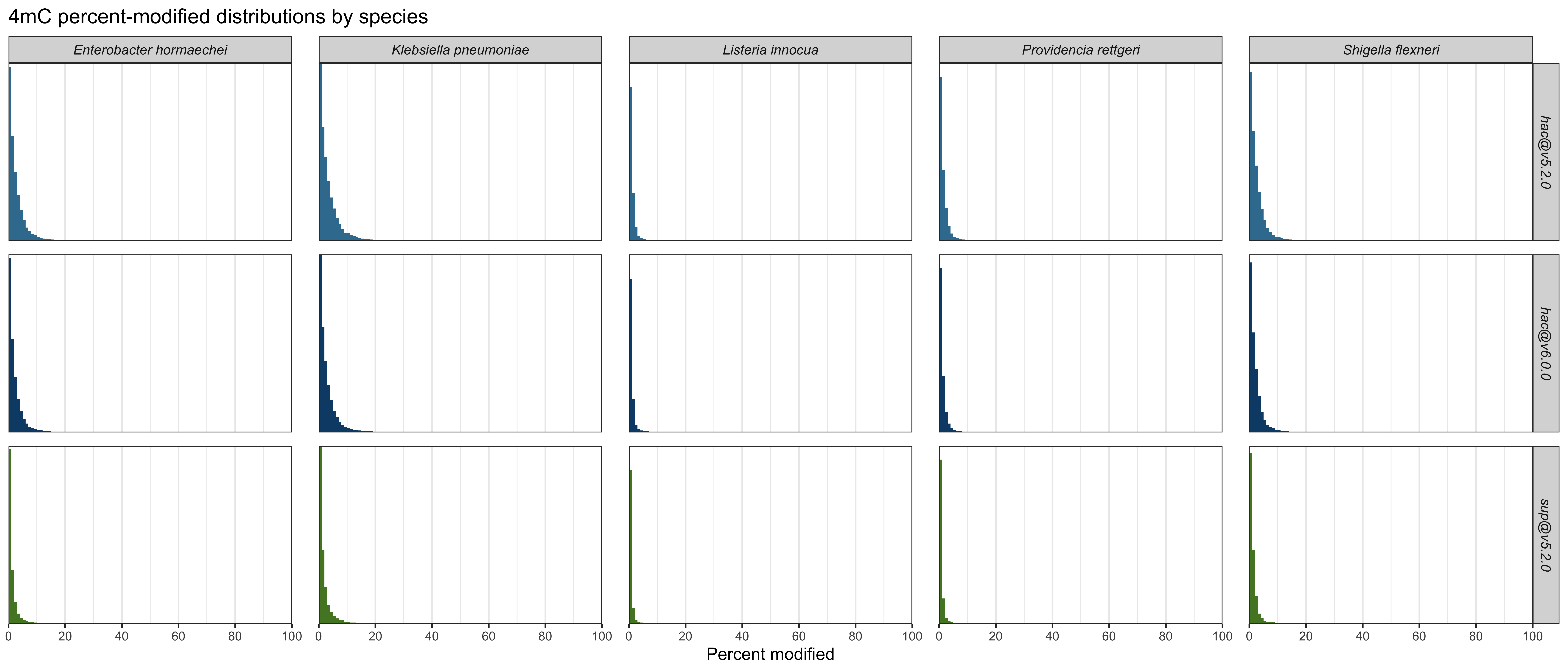
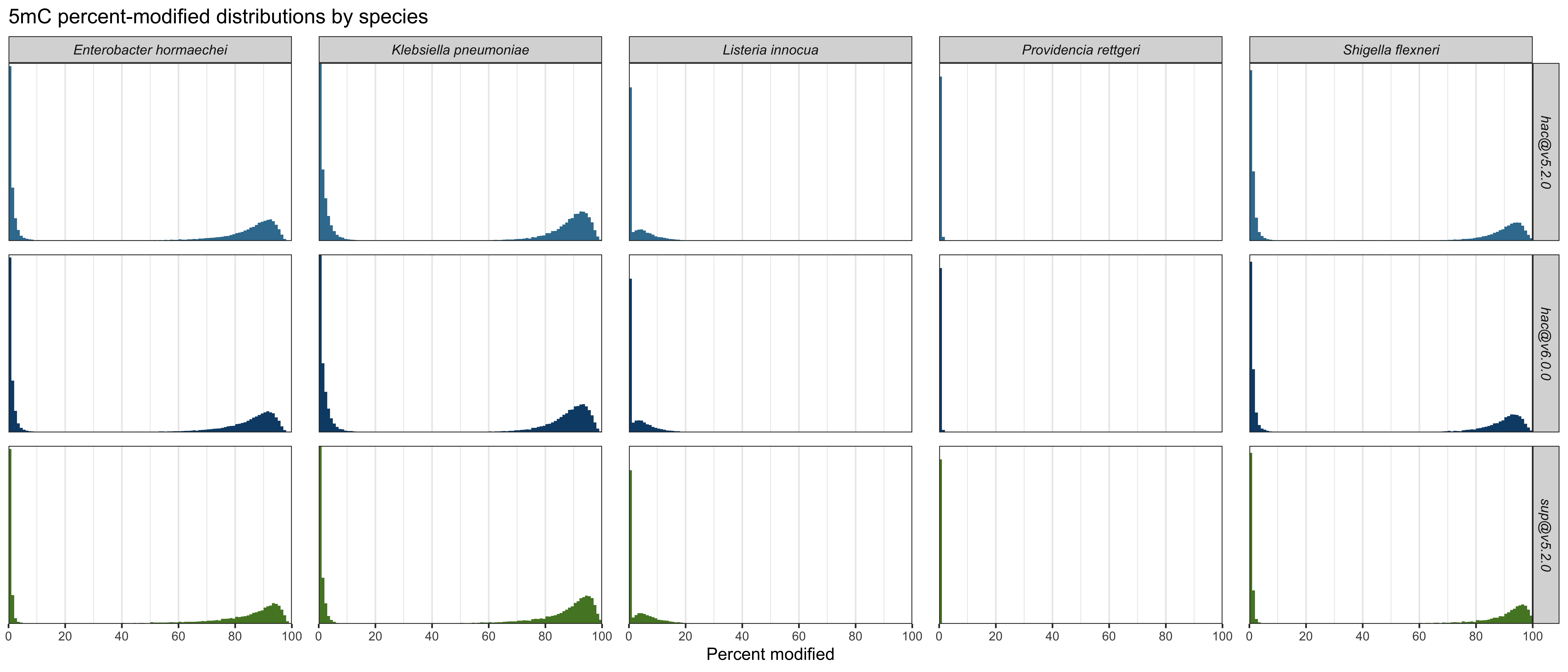
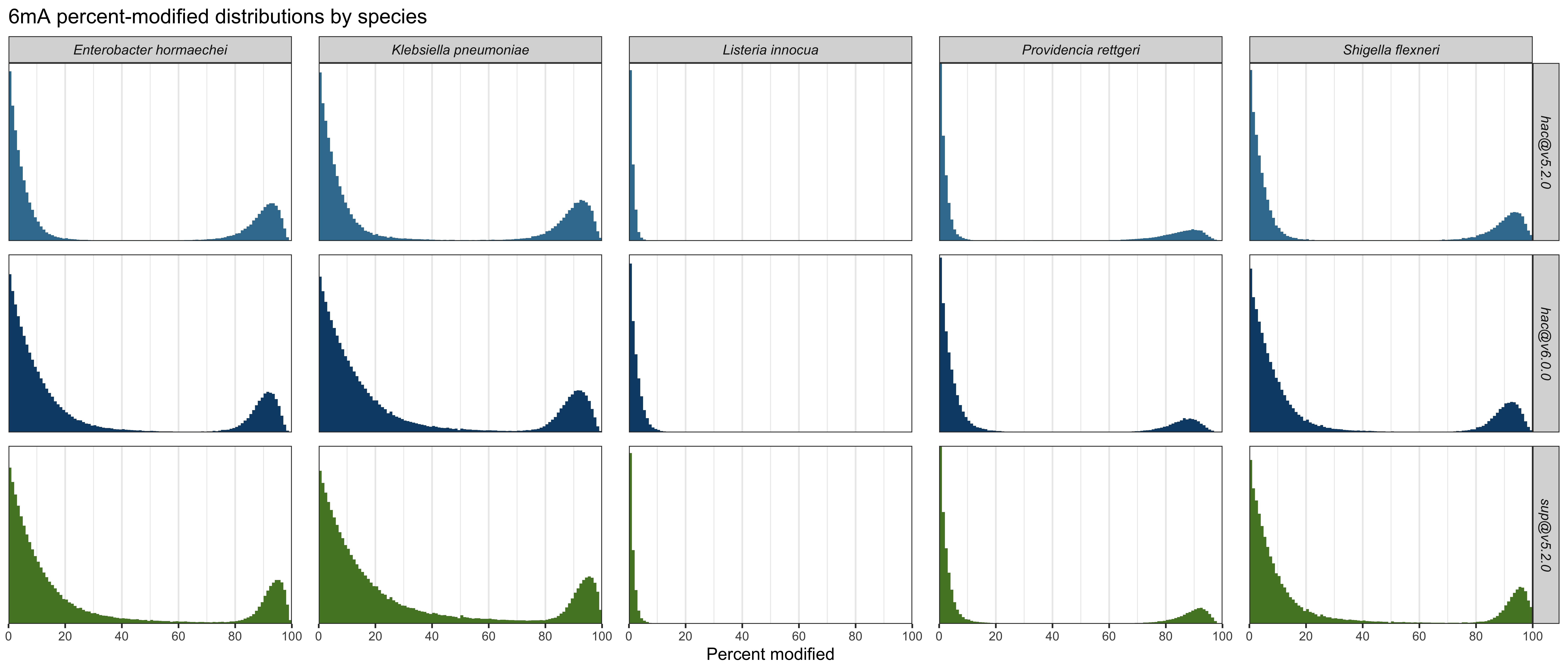
Discussion and conclusions
Going into this analysis, I was hoping that sup@v5.2.0 would always do best, as that would make my basecaller recommendations nice and simple. But the results were more complex and sometimes confusing. The best-performing basecalling model seemed to be either hac@v5.2.0 or sup@v5.2.0, depending on the metric. This contained two surprises: that hac@v6.0.0 did not always outperform hac@v5.2.0, and that hac@v5.2.0 sometimes outperformed sup@v5.2.0. And the inconsistent results for 5mC are strange, specifically how sup@v5.2.0 looked strong on low-peak mean and high-peak mean but seemed to have poor recall for CCWGG (a result consistent across all three genomes with that motif).
Overall, I think my recommendation from the last two posts is still mostly true: for ONT bacterial genomics, users should stick with sup@v5.2.0 basecalling. But with a possible caveat: for some analyses focused on 5mC, hac@v5.2.0 might be best. For example, if your downstream application cares about sensitivity (i.e. missing a modified position would be bad), hac’s better recall could matter.
All that being said, this mini-study has a lot of limitations. I had no ground truth so needed to quantify the ‘best’ model indirectly. My ‘Mid-range %’ metric can’t distinguish a genuine calling error from real intermediate methylation. My genomes contained no 4mC methylation, so performance there is still unclear. I also did not use the predicted modification probabilities in a sophisticated way – I just relied on the default modkit behaviour to distil each position of each read into a binary methylated-or-not call. So I am open to seeing new data and deeper analyses which might change my mind!
Over these last three posts, I’ve been fairly critical of hac@v6.0.0: ONT claimed it’s as good as (or better than) sup@v5.2.0, but my results have not supported this. My guess is that hac@v6.0.0 was developed with a focus on human sequencing, and if I had run my analyses on human data, the results may have looked more favourable for hac@v6.0.0. Zooming out, ONT’s bacterial WGS accuracy has largely plateaued over the last couple of years. Is that because the remaining errors are genuinely intractable? Or has ONT’s R&D effort been focused on human genomics at the expense of microbial genomics?
Footnotes
-
In this post, I use ‘methylation’ and ‘modification’ somewhat interchangeably. The modifications I look at here (6mA, 5mC and 4mC) are all base methylations, but not every DNA mod is. ↩
-
The slide on modified basecalling and this quote are at the 42:00 point. ↩
-
modkit motifclassifies motif instances into one of three sets (high-modified, mid-modified and low-modified) based on the bedMethyl fraction modified value. Whenmodkit motifproduces itsfrac_modvalue, it uses H/(H+L), i.e. it discards the mid-modified counts. In my numbers above, I used H/(H+M+L), i.e. I put all counts in the denominator. ↩ -
For
hac@v6.0.0, ONT claims 99.6% accuracy for 6mA and 98.6% accuracy for 4mC/5mC. ↩ -
All plots have a pseudo-log-transformed y-axis (count), which makes low-count regions more visible. ↩