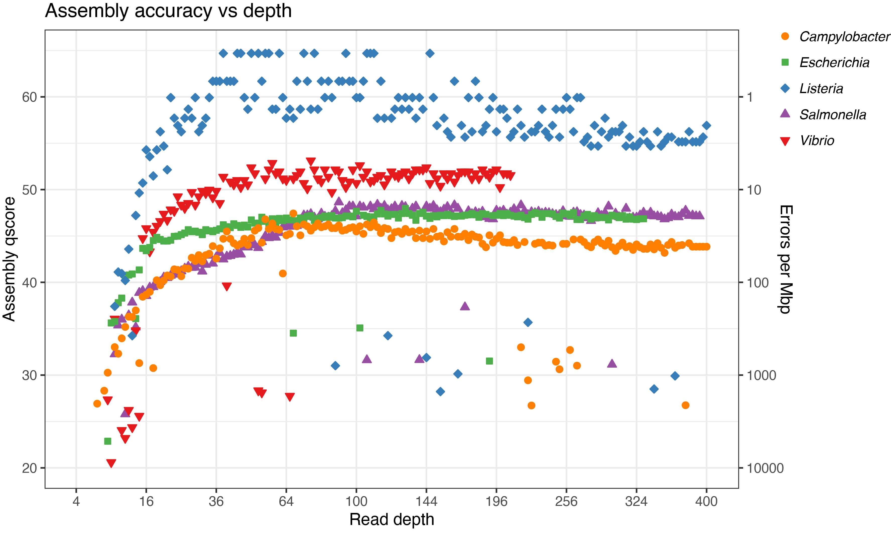
ONT accuracy vs depth update
After my last post, a common question arose (I’m paraphrasing):
Those accuracy values are interesting, but they came from very-high-depth Trycycler assemblies. What sort of accuracy could I expect for a normal-read-depth Flye assembly?
It’s a good question which I hope to address here. Consider this something of a sequel to my 2021 accuracy-vs-depth analysis.
Methods
Instead of using all nine genomes from my last post, I used just one genome per genus1:
- Campylobacter jejuni (ATCC-33560)
- Escherichia coli (ATCC-25922)
- Listeria monocytogenes (ATCC-BAA-679)
- Salmonella enterica (ATCC-10708)
- Vibrio parahaemolyticus (ATCC-17802)
And I only used the sup-basecalled reads (dna_r10.4.1_e8.2_400bps_sup@v4.2.0) from my last post for this analysis. While the fine-tuned bacterial research model did a little bit better, I thought I should stick to a standard Dorado model to make these results more relevant.
For each genome, I used the Trycycler-partitioned reads for the largest replicon2, which simplified the assembly and analysis: each read set should cleanly assemble into one circular contig. I then used seqtk to produce 200 random subsamples for each read set with depths ranging from 0× to up to 400× (uniformly spaced on a square-root scale).3 I assembled each with Flye v2.9.2, took the largest contig and rotated it to a consistent starting position with Dnaapler. I didn’t polish with Medaka.4 I then counted the differences5 between each assembly and the Illumina-polished ground truth I made previously.
Results

This table compares the peak6 Flye accuracy to the Trycycler accuracy (from my last post):
| Genome | Flye | Trycycler |
|---|---|---|
| Campylobacter jejuni | 42.65 errors Q46.2 |
27 errors Q48.2 |
| Escherichia coli | 91.60 errors Q47.5 |
70 errors Q48.7 |
| Listeria monocytogenes | 1.25 errors Q63.7 |
0 errors Q∞ |
| Salmonella enterica | 71.75 errors Q48.2 |
8 errors Q57.8 |
| Vibrio parahaemolyticus | 19.70 errors Q52.2 |
7 errors Q58.7 |
Discussion and conclusions
First, it’s important to keep in mind that these read sets were very clean and assemblable. This is because they already went through QC and Trycycler partitioning7 – there were no short or junky reads, so every read was in principle valuable for the assembler. That means a 100× depth set in this analysis might be equivalent to a real-world 150× set, because after throwing out short and low-quality reads, you could lose 1/3 of your data.
That being said, I was still impressed with Flye. It often gave a decent assembly at very low depth (<20×). And it only produced a large-scale error in ~5% of its assemblies (the low points in the plot), i.e. ~95% of the assemblies were structurally perfect, containing only small-scale errors.
You can see in the plot that accuracy improved up to ~100× depth, after which additional reads brought no benefit. In fact, some of the genomes got a bit worse with higher depth, which was surprising.8 This suggests that if you have very-high-depth read sets, subsampling them (e.g. with Filtlong) before Flye assembly might benefit not just computational time but also sequence accuracy. But I want to stress that these results are specific to Flye and its consensus algorithm. Different assemblers (e.g. Canu) would likely produce different accuracy-vs-depth curves that may not have this dropping-off-at-higher-depths effect.
While >100× depth didn’t help with assembly accuracy in this test, there are still benefits to deep ONT sequencing. Deep read sets allow for more aggressive read-length filtering9 and they help with Trycycler assembly. Notably, for each genome, the peak accuracy in this analysis was worse than the Trycycler accuracy in my last post. So when accuracy really matters, I still recommend sequencing to a depth of 200× or more and assembling with Trycycler.
Footnotes
-
This saved some computational time. Also, the accuracy values within each multi-genome genus were reasonably consistent, so I didn’t think including all nine would add much. For Vibrio, I kept V. parahaemolyticus – this is because V. cholerae had a long inverted repeat in its chromosome that made it tougher to assemble. For Campylobacter and Listeria, I kept C. jejuni and L. monocytogenes because they are the more commonly studied species. The five genomes I used here are the same ones from my May post. ↩
-
For most genomes, the largest replicon was the chromosome, and for the Vibrio genome, it was the larger of the two chromosomes. ↩
-
Only the Campylobacter and Listeria genomes had >400× depth, so for the other three, I took the depth as high as I could go. Vibrio was the shallowest with only 208× depth to work with. ↩
-
I skipped Medaka both to save time and because it doesn’t seem to help much for sup-read assemblies. ↩
-
I used my
compare_assemblies.pyscript to get a difference count. ↩ -
To calculate peak accuracy for each genome, I used the mean error count from the 20 best assemblies. ↩
-
The reads were first QCed with Filtlong:
--min_length 10000to remove short reads then--keep_percent 90to discard the worst 10% of each read set. Then Trycycler partitioning served as an additional QC step, because any read which originated from something else (e.g. a plasmid or cross-barcode contamination) was discarded. ↩ -
Note that my read subsampling was random (
seqtk sample), so lower depth sets did not have a higher average quality (as would have been the case if I had used Filtlong to subsample). ↩ -
For example, if you have a very deep read set, you can throw out all reads <10 kbp and still have plenty left over. This generally makes assembly easier, though small plasmids can be lost. ↩
